Loadcells
Measuring displacement of a point or surface, rather than measuring the deformation of a flexure, offers many possibilities for compact, low-cost load cells. This page gathers some resources on this topic and presents work towards a simple six degree-of-freedom (DOF) loadcell based on these ideas.
Capacitive
One way to determine the proximity of two surfaces is by measuring the capacitance between them. This page documents experiments with a 3 DOF Capacitive load cell using a single printed circuit board.

It is based on a discrete electrostatics solver (shown below), and also documented on the page above.
Magnetic
Another position measurement uses the magnetic field instead of the electric field. Among magnetic field sensing technologies, hall effect sensors are the most ubiquitous. Integrated circuits with arrays of hall effect sensors are available at extremely low cost in very dense packages. Using differential pairs of these elements, non-contact rotary and linear encoders can be made. A great resource for designing such magnetic devices is the Honeywell Hall Effect Handbook. Austrian Microsystems makes a variety of these devices for sensing position or rotation of a magnet.
For more sensitive, low field devices magnetoresistive sensing elements are often used. David Pappas of NIST compares noise floors of these technologies, noting hall effect sensors register around 300,000 pT/\sqrt{Hz}, while magnetoresistive 200
Integrated circuits are available with extremely sensitive magnetoresistive and hall effect sensors.
AS5510 1 DOF Loadcell
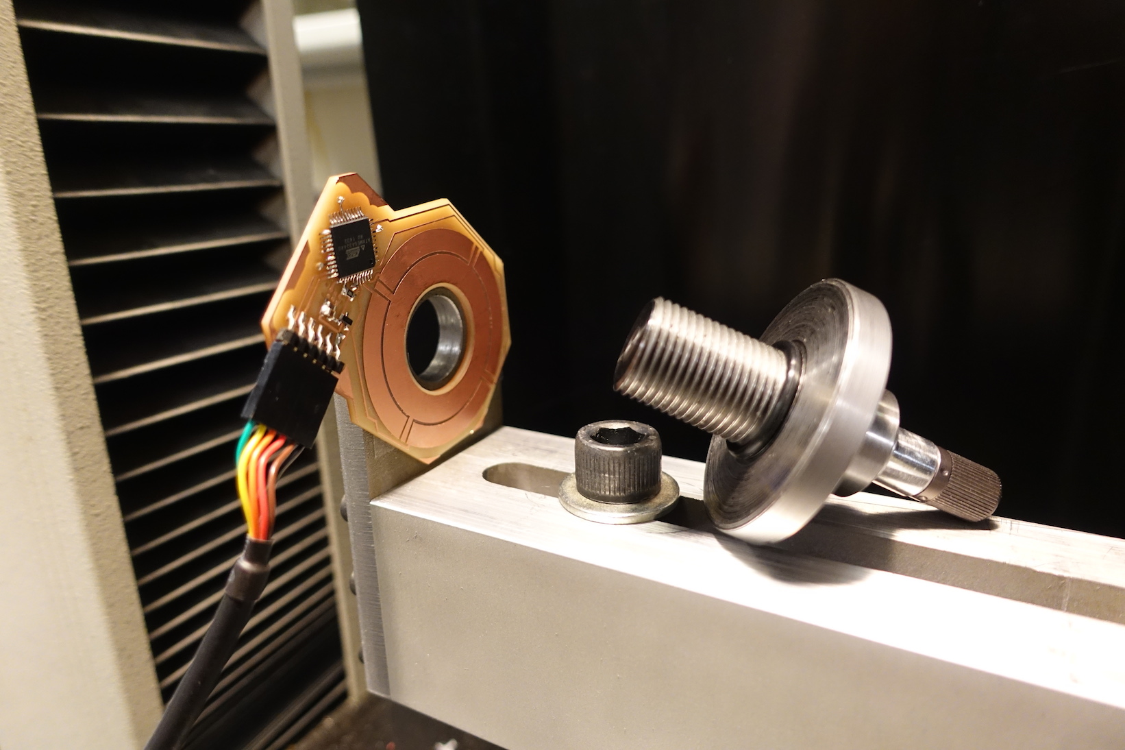
Here, we document experiments with a 1 DOF magnetic load cell, based on the Austrian microsystems AS5510 10 bit linear encoder IC, which boasts 500nm resolution for $1.41 (Q: 100).
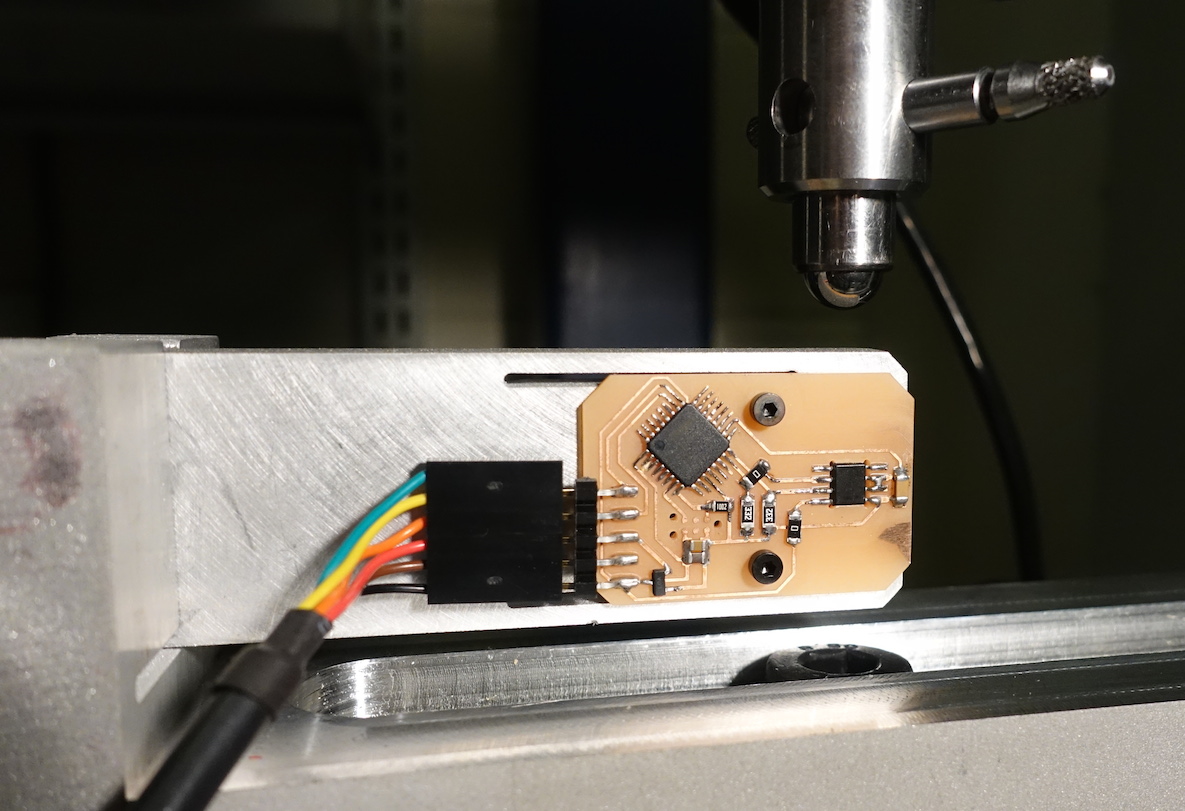
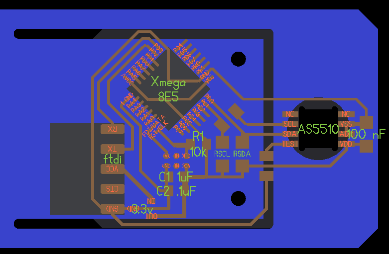
The PCB is mounted to a piece of waterjet aluminum with a flexure cut into it. A magnet sits in a hole on the moving part of the flexure. I designed the flexure to be roughly 5 um/Newton. The encoder wants a air gap of less than 1mm, so I milled away the board inside the SOIC-8 footprint and flipped the part over to bring it closer to the magnet underneath.
I'm using an 8mm circular diametrically magnetized magnet. We could swap in a smaller magnet to push the resolution of the prototype, but I started with the datasheet's recommended magnet form factor. I'm running the chip at its highest sensitivity (+-12.5 mT full scale) and in slow mode (12.5 KHz as opposed to 50 KHz, but .5 mT peak-to-peak noise as opposed to .8 mTpp).
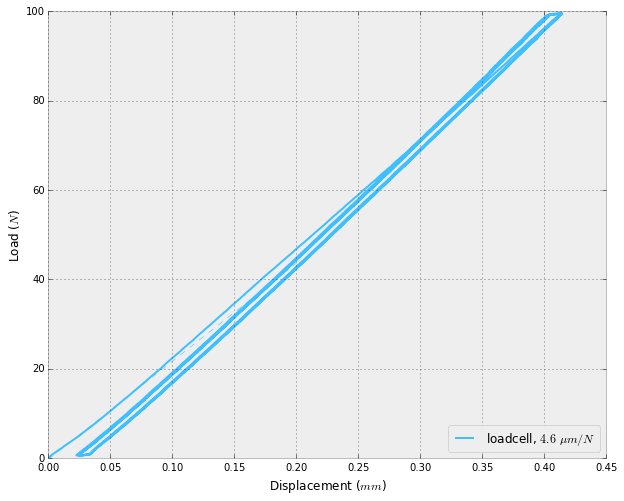
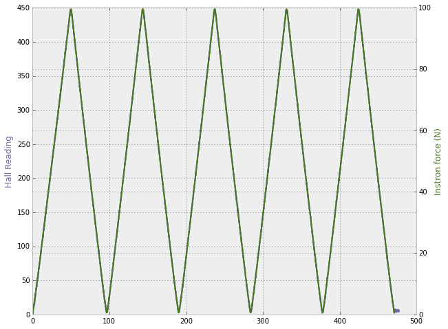
The graphs below show instron characterization of the prototype. First, the flexure had a stiffness of 4.6 um/N, close to the designed 5 um/N. Second, the time series comparison is very boring because the two series are so identical. We see that a displacement of 400 um (corresponding to 100N) takes the encoder nearly over its full range (512 is the full range, as it measures positive and negative displacement to 10 bits (1024)).
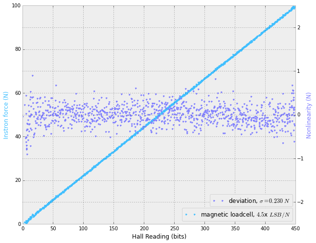
Finally, we can plot the relation between the two variables (force and hall reading). Running at the full 12.5 kHz (i.e., without any summing of samples), we get about 5x LSB per Newton. This isn't amazing resolution, but it is very much good enough for my application. Further, we can easily take a hit in speed to get an increase in resolution by summing (i.e., averaging) samples, depending on the applciation.
6 DOF Loadcell
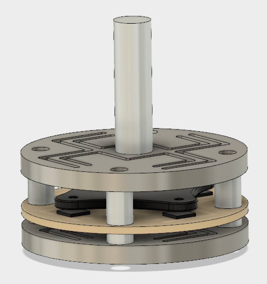
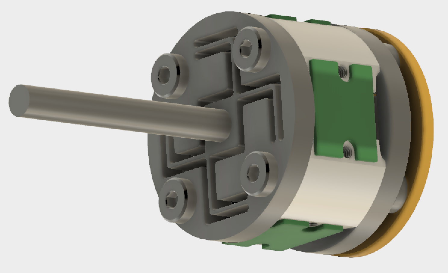
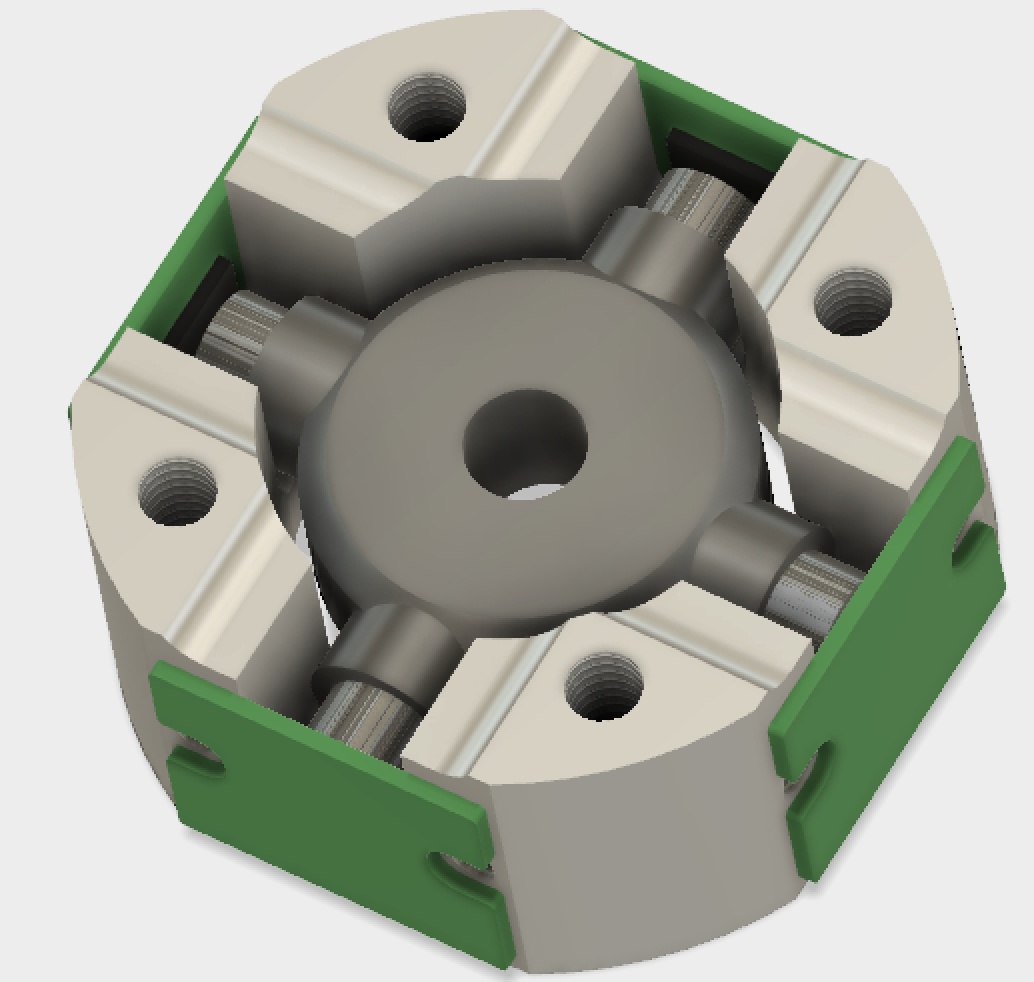
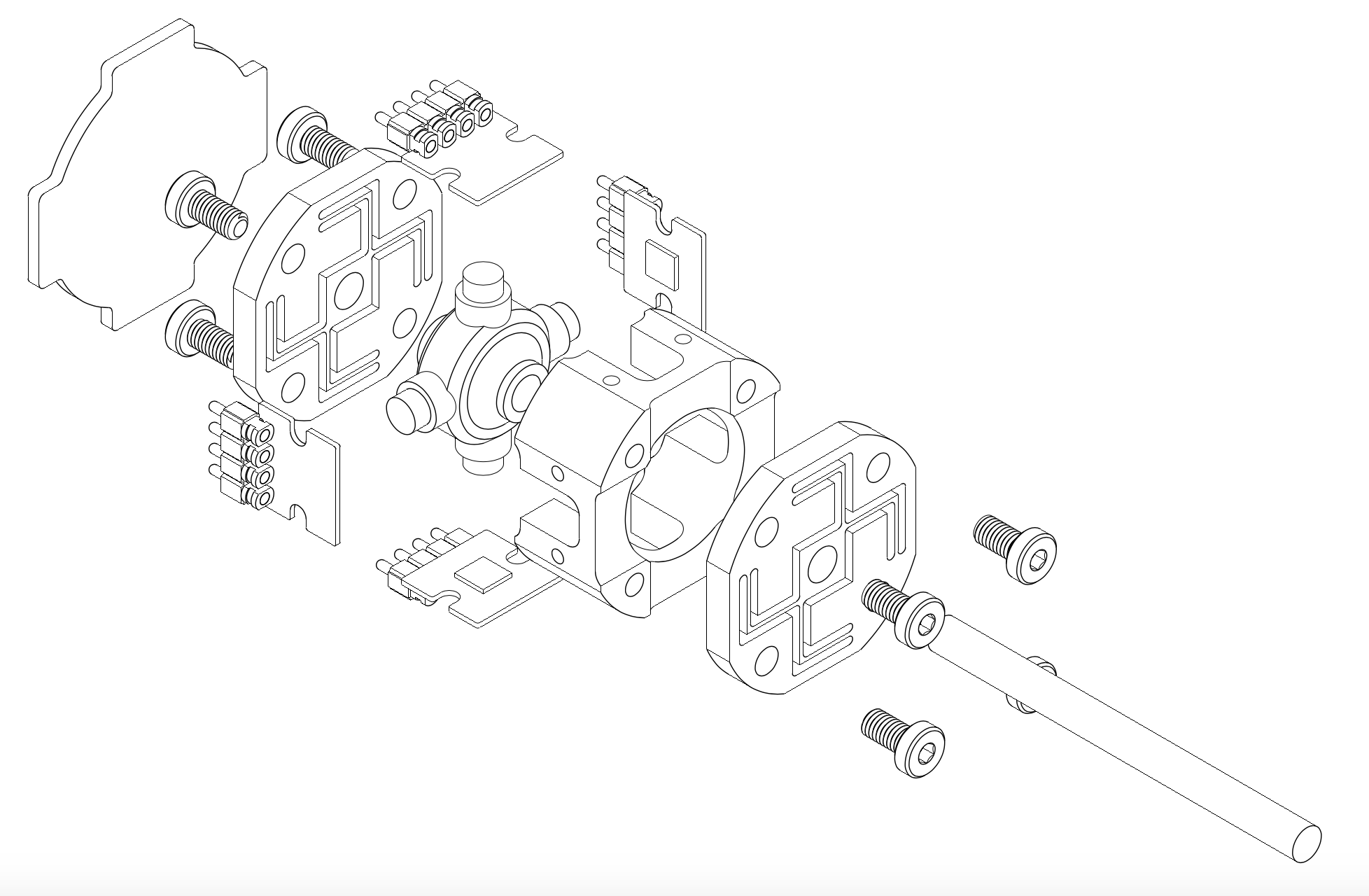
A concept for a 6 degree of freedom magnetic load cell is shown below. It uses a pair of flexures (aluminum or titanium plates on top and bottom) to set relative stiffnesses of Fx, Fy, Fz, Tx, Ty, Tz. A central rod carries a disk with four small neodymium magnets which moves when loads are applied. Four AS5013 hall array ICs are positioned just below the rest positions of the magnets on a single PCB. M3 standoffs and screws hold the entire stack together.
Features of a "good" 6 DOF flexure:
- Ability to tune relative stiffnesses (e.g. Fx/Fz, Tx/Tz, etc.)
- Minimal cross talk (e.g. Fx doesn't induce a displacement in y or a twist, etc.)
- Fits into a reasonably small bounding volume.
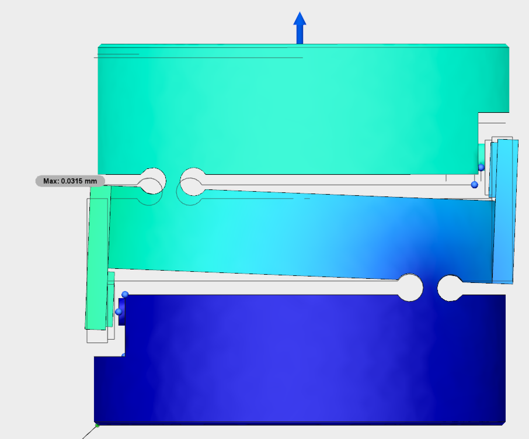
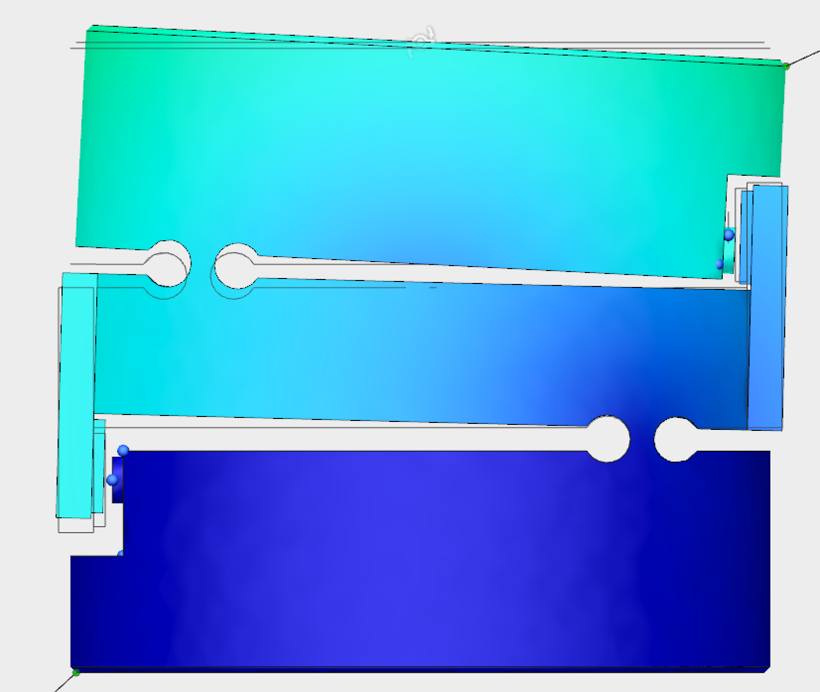
Fusion 360 lets us quickly test loading cases for flexure designs. Below are simulations of a force and a moment applied to the loadcell.
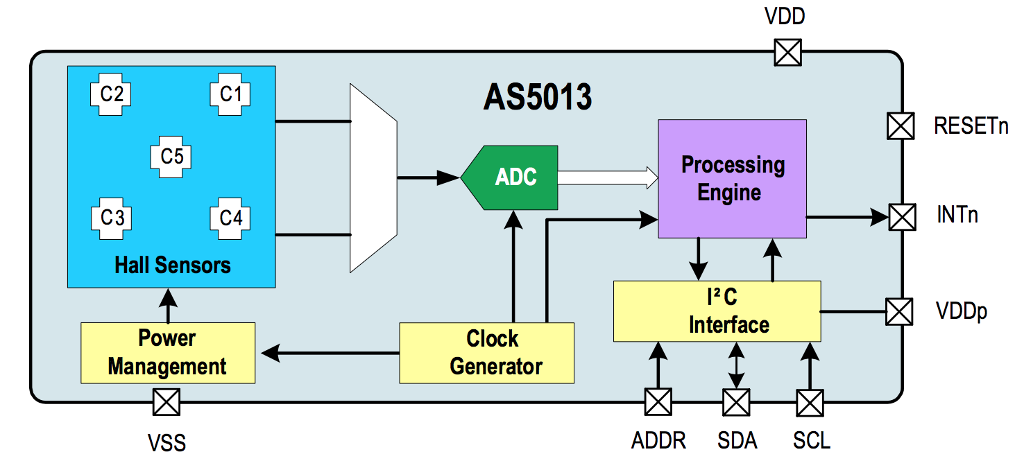
Building on the experiments with the AS5510, we explore the use of the AS5013 ($4.42 in Q100) to perform 3-dimensional tracking of a magnet. This IC is nominally an 8-bit 2 axis magnetic encoder, though it contains 5 hall effect sensors, each with 12-bit resolution, adjustable gains, and I2C-accessible raw values. as5013-test/ contains pcb source files for a board to evaluate this measurement.
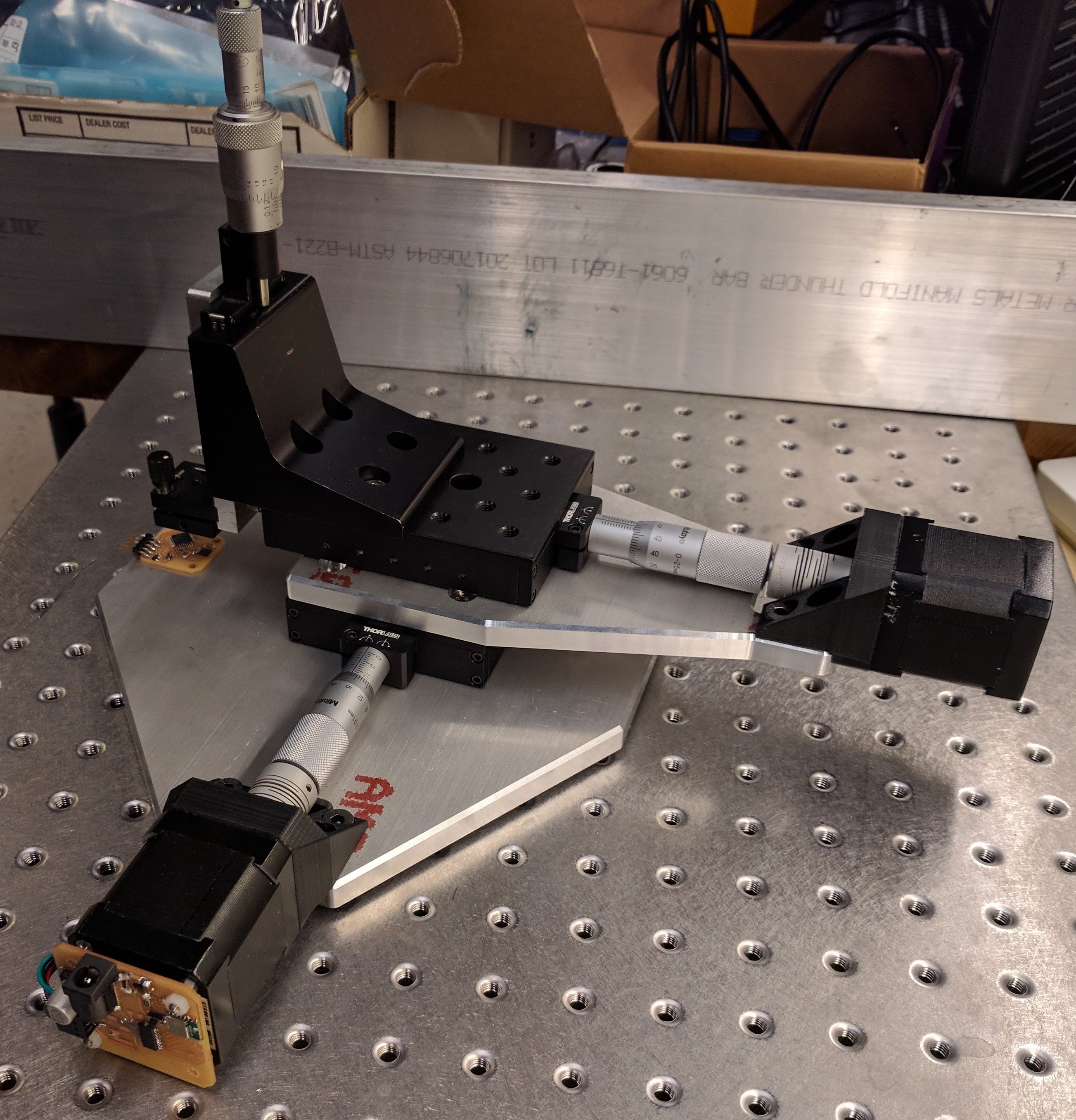
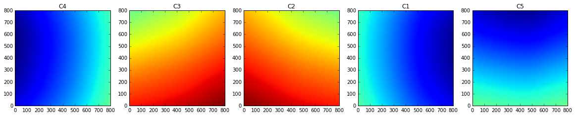
To characterize the use of the AS5013 as a three-dimensional tracking device, we use a 5 axis stage (2 axes motorized, 3 manual) built around two Thorlabs PT1M micrometer stages. After setting a magnet height and orientation, we can sample the 5 hall elements over a two dimensional array of magnet displacements. Executing this for a handful of magnet heights should let us fit functions for X, Y, and Z in terms of the 5 hall readings.

Below are some preliminary plots of readings from the 5 internal hall effect sensors. They each run over 800 um with 10 um sample spacing.
 If we scan over a broader area, we can start to see deviations from an ideal radially symmetric field (there is also an overflow error in these plots that I haven't fixed yet).
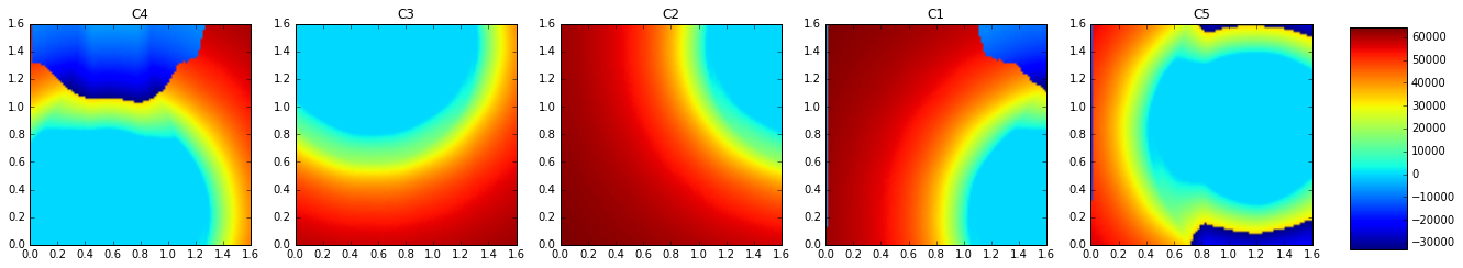
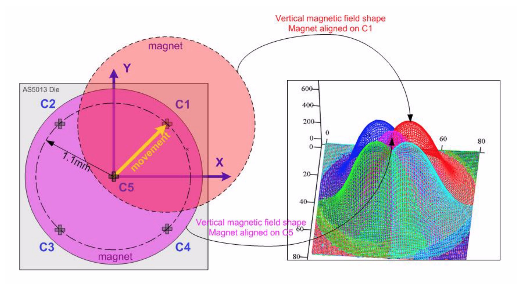
This last plot indicates why the magnet spacing is 1.1mm -- from the center of the magnet, this is the approximate distance to the highest gradient in the z component of magnetic field. This observation leads us to consider if we want to maximize resolution in tracking the magnet, could we make an alternative arrangements of magnet(s) to produce higher field gradients.
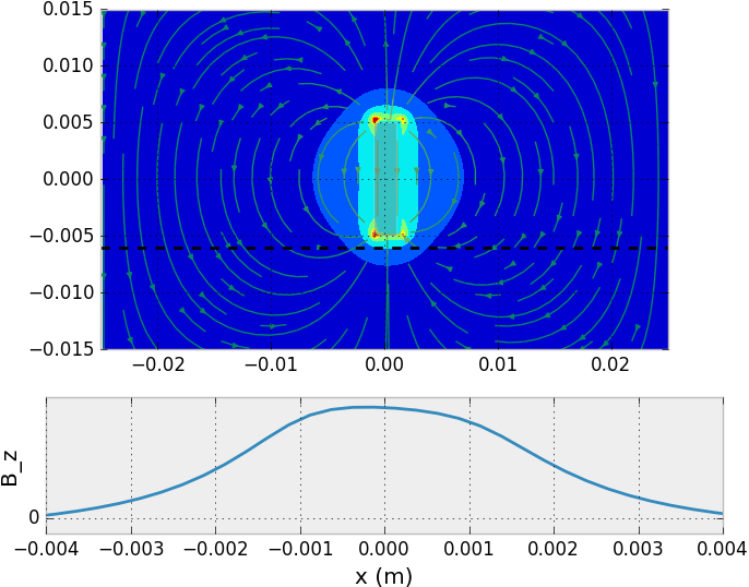
To test this, I wrote a very simple (and slow for now!) 2D B field finite difference simulation, which is in sim. It uses successive overrelaxation to compute the spatial distribution of the z component of the magnetic field (todo: fix the field magnitude bug here). Below we should output of the simulation for a single magnet, as well as for a pair of opposing magnets. The first plot roughly confirms the shape and size of the magnetic field funtion from a single rod magnet.
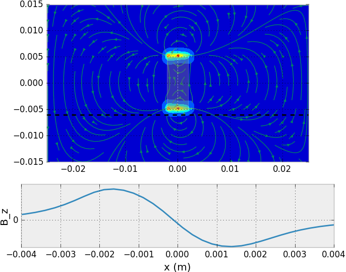
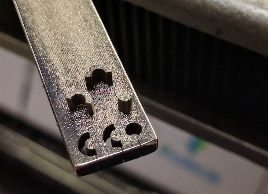
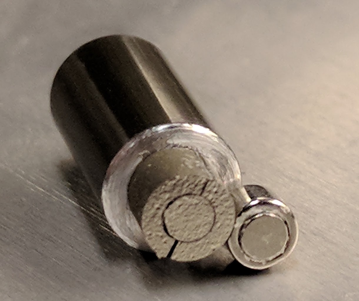
The pair of opposing magnets produces a high field gradient. We could create such a region of high field gradient over each of the four outer hall effect sensors using a simple arrangement of a central magnet with a surrounding annulus of opposite polarity. I EDM'ed a test arrangment out of a large neodymium magnet of 1/8" thickness. This went reasonably well, except for a small tab near the lead-in which was left due to the brittleness of the magnet material.
I put this magnet arrangement on my stage to test the resolution. I just grabbed the 8 bit X and Y values computed by the AS5013 and looked for the spatial range this mapped over. Below are some very preliminary plots of this data, having not changed many of the parameters for the calculations.
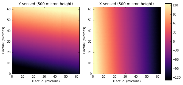
This we extremely encouraging: we improved the resolution of this linear encoder to have a LSB of ~200nm!
I switched the stage into 1/8th microstepping mode (nominally 156 nm / step, but subject to backlash, etc.), and pulled out the raw sensor values. We can create simple shape functions for the x and y displacement values as
Evaluating these, we can create the graphs below:
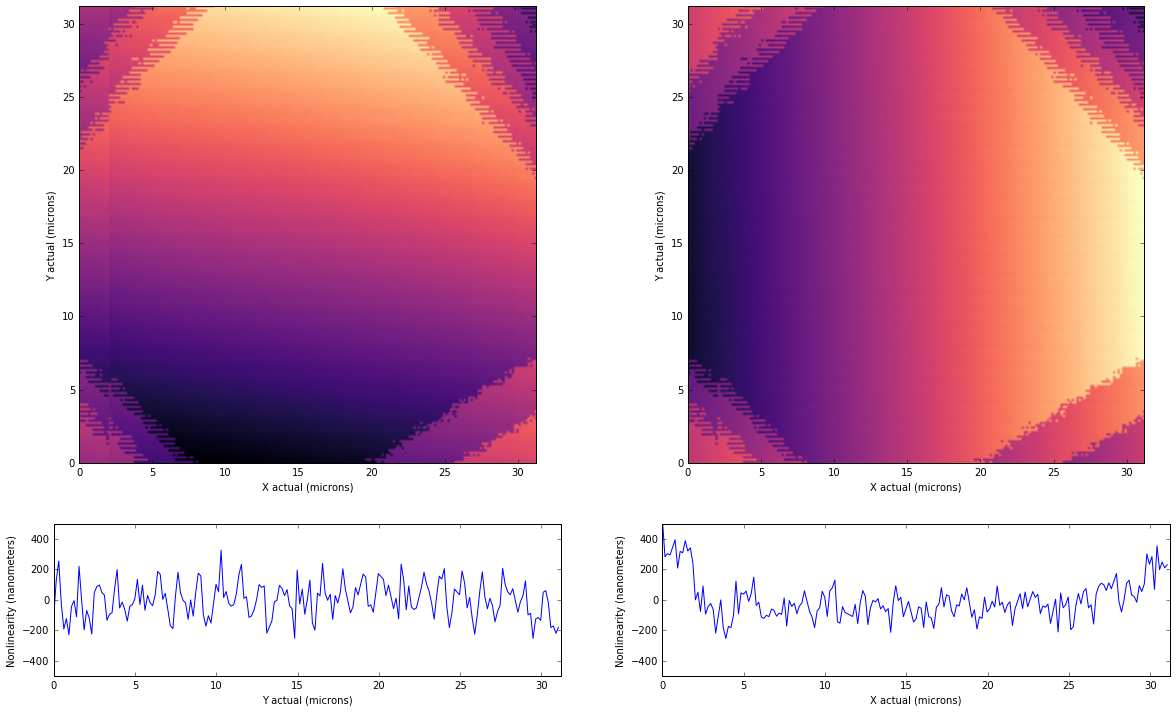
These measurements are pulled from a single measurement on the sensor, so I expect averaging will reduce some of this nonlinearity. I also want to play with the sensor gains to increase the region before the internal ADC overflows. The goal of this will be to maximize dynamic range, which we could evaluate as the ratio of full scale to the standard deviation of the nonlinearity. In the simple measurements above, this dynamic range is roughly 8 bits. If we oversample 16x, we can get 10 bits at 150 Hz. If we turn down the gains, we may work further above the hall elements' noise floors, additionally increasing dynamic range. We also can turn on hall element
These measurements are also just at the edge of the positioning we can expect from our stage. In fact, we can see the limits of stage repeatability in the graph at left, where an artifact shows at the left due to overscanning the grid and the misalignment between consecutive scans. This ramifies in the nonlinearity measurement of the
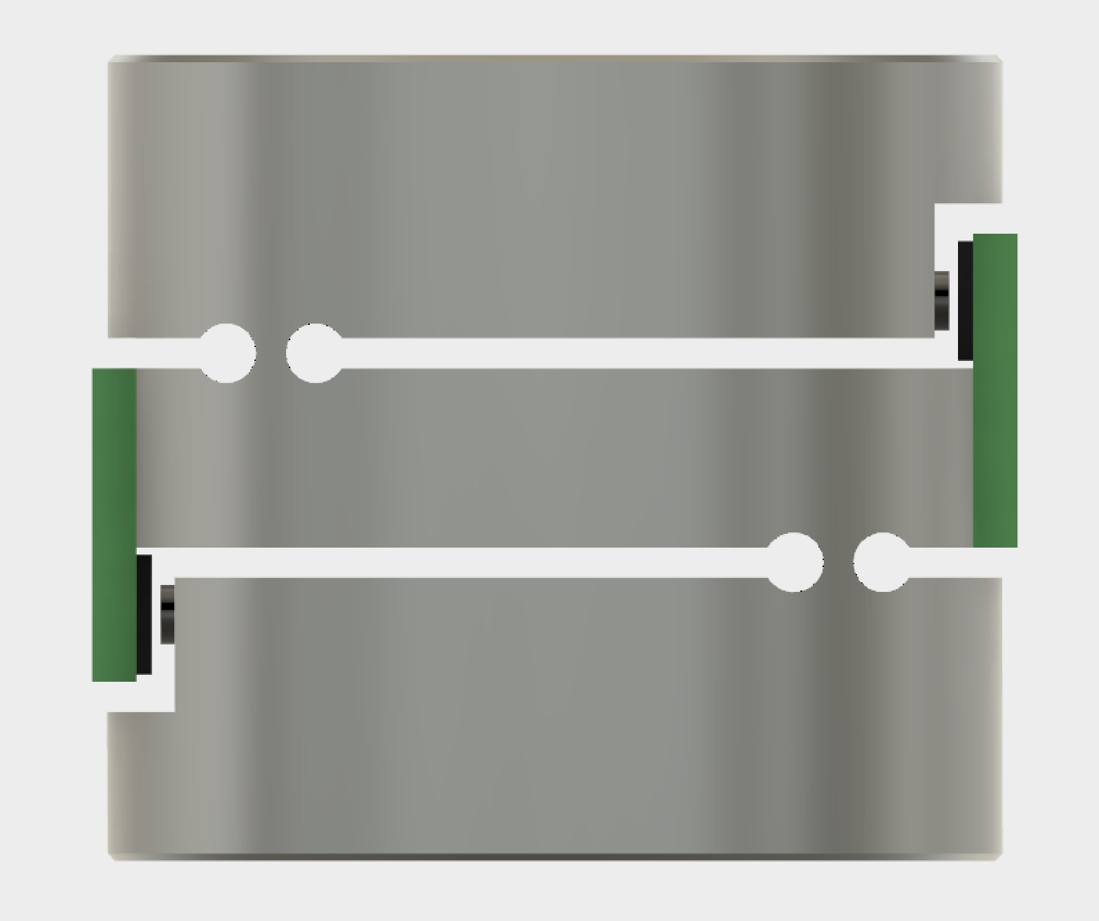
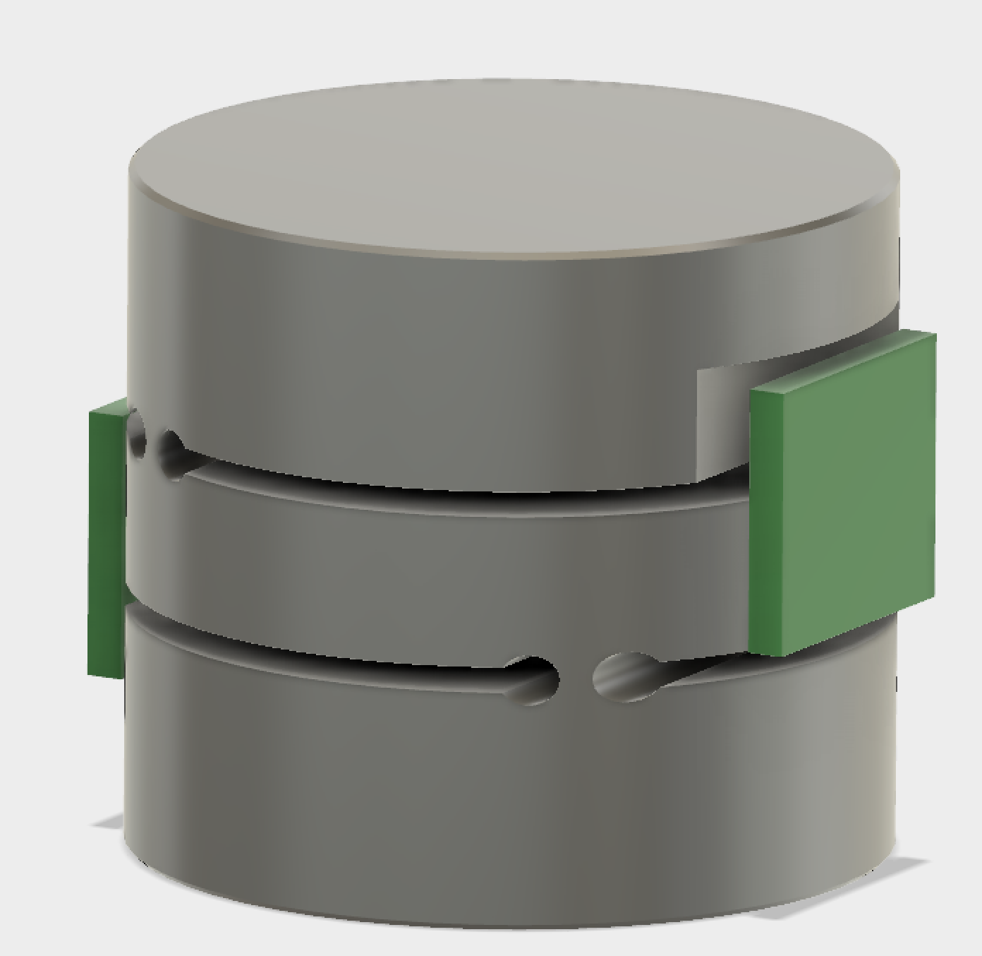
Below we show a new design incorporating this magnet change and rotating the ICs to give differential measurements in all axes.
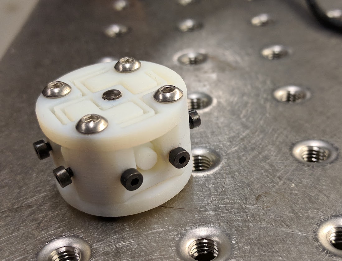
I did a quick 3D print of this design to check clearance and assembly issues. The flexure looks great (albeit obviously too compliant in the photopolymer material).
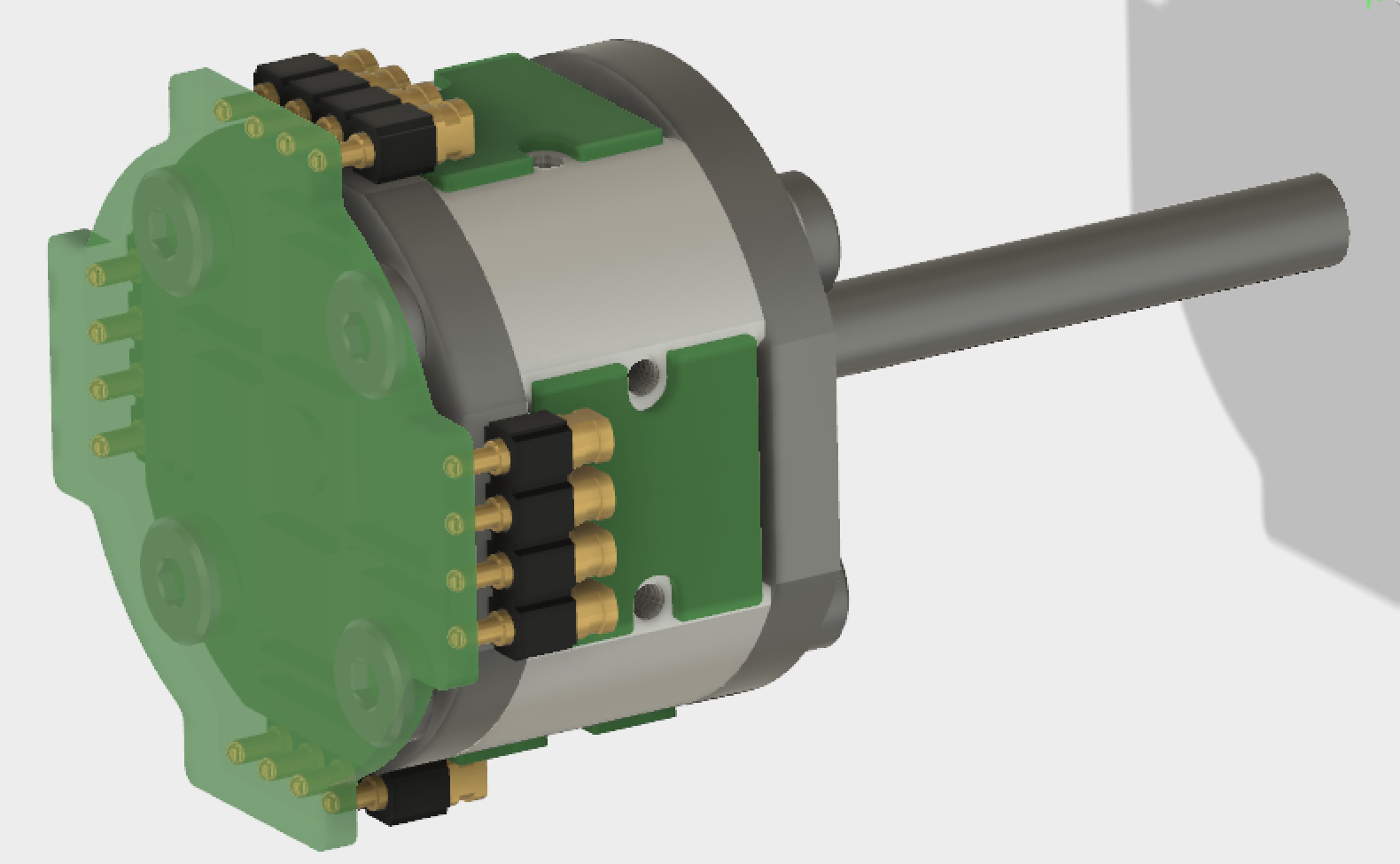
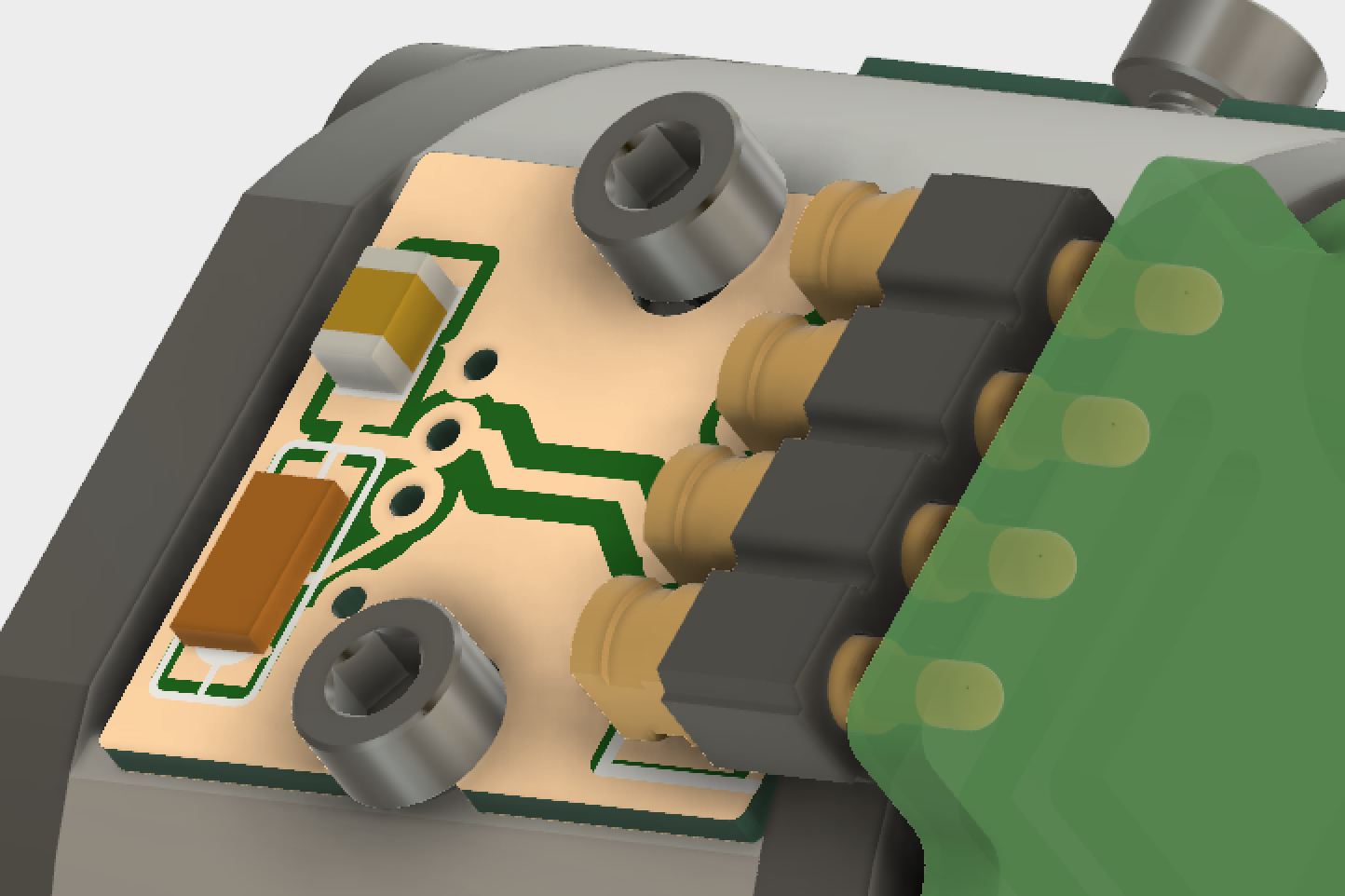
Next task is designing the AS5013 board and its connection to the main board on the end of the cylinder. I'm thinking of using the four position Mill-Max spring contact connectors to save space over a wired connector. It should make a solid electrical connection for the I2C lines, power, and ground, while allowing room for fine adjustments of the sensor carrier boards. It's going to be a tight fit getting around the corner.
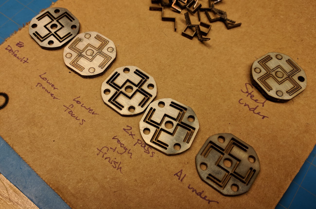
I prototyped the flexure out of .090" 304 stainless using our new FabLight 3kW fiber laser system. The cut was much cleaner than I expected, and I may have to use this tool rather than spend hours at the EDM.
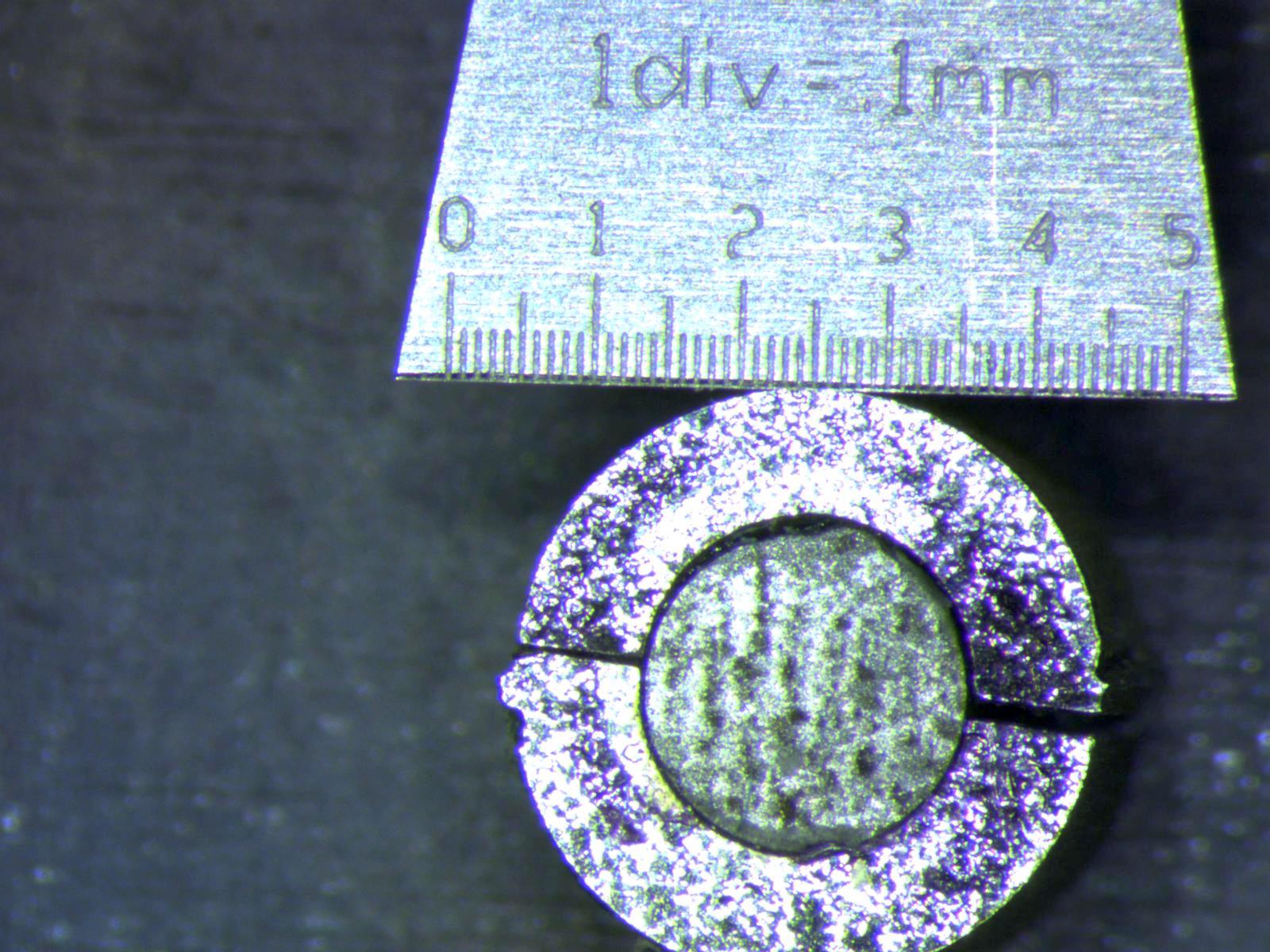
I also managed to source cylinder and ring magnets of the appropriate dimensions from Super Magnet Man. This means we don't have to fabricate the concentric magnet pairs. Below is an image of the new concentric pair next to the one I EDM'ed.
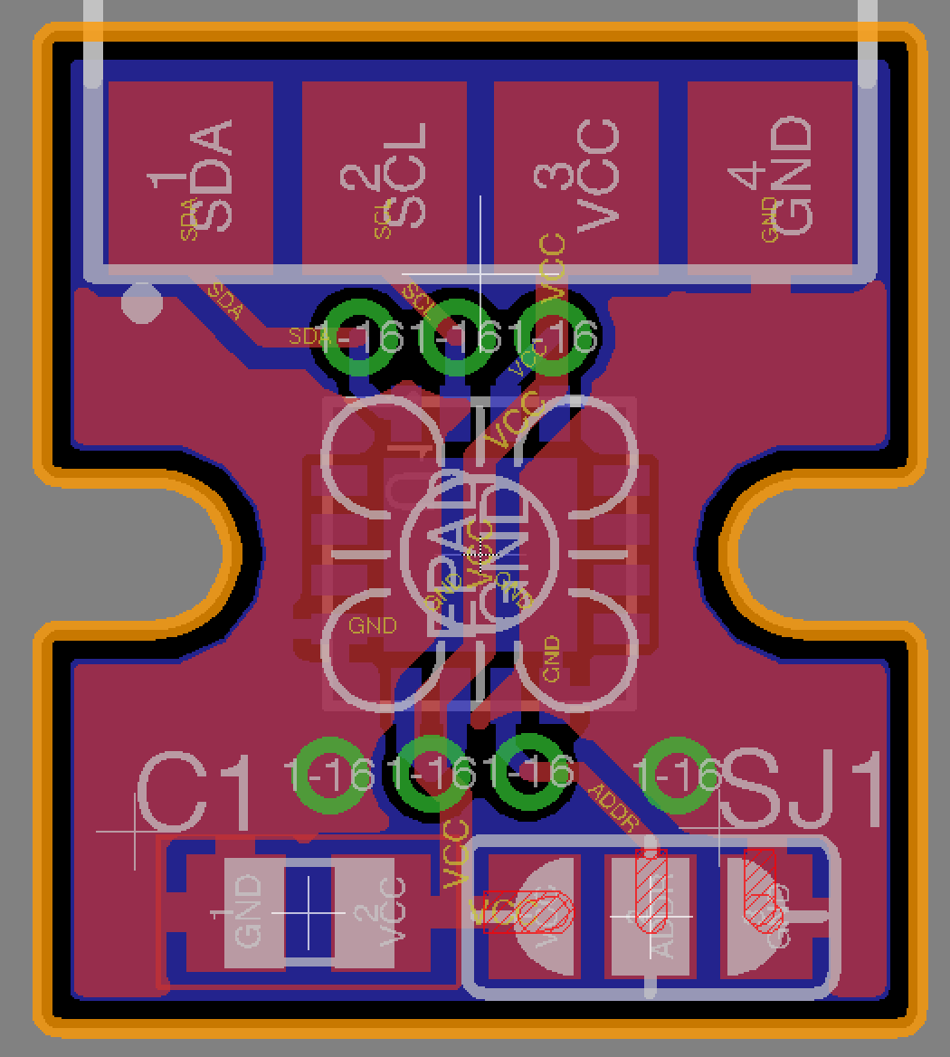
I designed the AS5013 daughter boards, using it as a chance to try the new integration of Eagle and Fusion360. It's still pretty rough, but I like where it's headed, and it was certainly useful for this purpose. I just grabbed the PCB outline geometry from Fusion, layed out my board in Eagle and pushed the changes back to Fusion to visualize the 3D circuit board in the context of my assembly. Below are both views. Pretty slick for "hobbyist cad"... My only complaints are that the appearances are a little rough in Fusion (the via pads don't really overlap...) and the syncing process can be a little buggy.
I'm sending out for a run of these boards which should allow me to experiment with calibration and measurement, both for the 6 DOF configuration, as well as others.
Torque Cell
I've also been looking at a similar mechanism for a non-contact torque cell. Most such torque measurement devices use a slip ring or radio telemetry to transmit the measured values to the stationary frame. We can design a flexure (similar to a helical shaft coupling) with a portion that translates in the axial direction when subjected to torque. Depending on requirements, we can dial up and down the stiffness and range. We can mount an axially magnetized ring magnet (or better yet, an opposite pair of ring magnets) and measure the axial displacement using a pair of differential hall elements in the stationary frame. This allows us to subtract out small deviations in the gap between the magnet and sensor. Below are some quick simulations of a candidate flexure geometry:
The video above shows a printed test of an exagerrated flexure (so that we can see the deflection). I've also printed some much stiffer flexures which translate in a range measureable by a differential hall effect pair.
2 DOF Force + Moment
After talking to Ian about the requirements of a 2 degree of freedom load cell for a prosthetic ankle application, here was a quick sketch of a flexure and layout of magnets and sensors.
The two sensors can differentiate forces in the Z direction and moments around the X axis (out of the screen).